Ordinals Explained

Why does the ordinal() function not reflect the ranks passed into rate()? Consider for instance the example below:

Let’s first install some packages we need.

%pip install openskill
%pip install pandas
%pip install matplotlib
%pip install numpy

# Import openskill.py and plotting libraries.
import matplotlib.pyplot as plt
import pandas as pd
import numpy as np
from scipy.stats import norm
from openskill.models import PlackettLuce

# Initialize Default/Starter Rating
model = PlackettLuce()
r = model.rating

Requirement already satisfied: openskill in /usr/local/lib/python3.10/dist-packages (5.0.1)
Requirement already satisfied: pandas in /usr/local/lib/python3.10/dist-packages (1.5.3)
Requirement already satisfied: python-dateutil>=2.8.1 in /usr/local/lib/python3.10/dist-packages (from pandas) (2.8.2)
Requirement already satisfied: pytz>=2020.1 in /usr/local/lib/python3.10/dist-packages (from pandas) (2023.3)
Requirement already satisfied: numpy>=1.21.0 in /usr/local/lib/python3.10/dist-packages (from pandas) (1.23.5)
Requirement already satisfied: six>=1.5 in /usr/local/lib/python3.10/dist-packages (from python-dateutil>=2.8.1->pandas) (1.16.0)
Requirement already satisfied: matplotlib in /usr/local/lib/python3.10/dist-packages (3.7.1)
Requirement already satisfied: contourpy>=1.0.1 in /usr/local/lib/python3.10/dist-packages (from matplotlib) (1.1.0)
Requirement already satisfied: cycler>=0.10 in /usr/local/lib/python3.10/dist-packages (from matplotlib) (0.11.0)
Requirement already satisfied: fonttools>=4.22.0 in /usr/local/lib/python3.10/dist-packages (from matplotlib) (4.42.0)
Requirement already satisfied: kiwisolver>=1.0.1 in /usr/local/lib/python3.10/dist-packages (from matplotlib) (1.4.4)
Requirement already satisfied: numpy>=1.20 in /usr/local/lib/python3.10/dist-packages (from matplotlib) (1.23.5)
Requirement already satisfied: packaging>=20.0 in /usr/local/lib/python3.10/dist-packages (from matplotlib) (23.1)
Requirement already satisfied: pillow>=6.2.0 in /usr/local/lib/python3.10/dist-packages (from matplotlib) (9.4.0)
Requirement already satisfied: pyparsing>=2.3.1 in /usr/local/lib/python3.10/dist-packages (from matplotlib) (3.1.1)
Requirement already satisfied: python-dateutil>=2.7 in /usr/local/lib/python3.10/dist-packages (from matplotlib) (2.8.2)
Requirement already satisfied: six>=1.5 in /usr/local/lib/python3.10/dist-packages (from python-dateutil>=2.7->matplotlib) (1.16.0)
Requirement already satisfied: numpy in /usr/local/lib/python3.10/dist-packages (1.23.5)

Let’s start with a simple case of what we know should work. Which is that ranks passed in will reflect the values of ordinals:

# Relevant Code
result = model.rate(teams=[[r()], [r()], [r()], [r()]], ranks=[1, 2, 3, 4])

# DataFrame Code
df = pd.DataFrame([_[0].__dict__ for _ in result])
df["ordinal"] = [_[0].ordinal() for _ in result]
df

	id	name	mu	sigma	ordinal
0	e2404cb87b1846fca9ccd6572d95a528	None	27.795253	8.263572	3.004537
1	f652af00058c423e92cd34575927427c	None	26.552918	8.179618	2.014064
2	0ea2b05f51e24e199ad789b71c86fe0c	None	24.689416	8.084128	0.437033
3	cf5f8d5f4bdb4ddb89aa7d7f6bfdbc4a	None	20.962413	8.084128	-3.289971

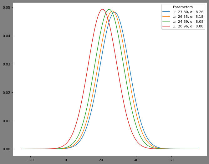
Let’s visualize the distributions of the 4 skills.

visualization_data = np.arange(-25, 75, 0.001)
fig = plt.figure(figsize=(10, 8), dpi=80)
fig.patch.set_facecolor("grey")
df.apply(
    lambda row: plt.plot(
        visualization_data,
        norm.pdf(visualization_data, row["mu"], row["sigma"]),
        label=f"μ: {row['mu']: 0.2f}, σ: {row['sigma']: 0.2f}",
    ),
    axis=1,
)
plt.legend(title="Parameters")

<matplotlib.legend.Legend at 0x79208ed09450>

You may have already noticed from the distributions of the system’s assesment of playeys skills that the lower ranked players are shifted from to the left from the mean.

Let’s try visualizing an edge case. First let’s see the ordinals from a tied game with 5 players

# Relevant Code - 5 Players with Ties
result = model.rate(teams=[[r()], [r()], [r()], [r()], [r()]], ranks=[1, 2, 3, 2, 4])

# DataFrame Code
df = pd.DataFrame([_[0].__dict__ for _ in result])
df["ordinal"] = [_[0].ordinal() for _ in result]
df

	id	name	mu	sigma	ordinal
0	ac2c7220bbd94a3db89adedda04ae55d	None	27.666827	8.290970	2.793916
1	ce0be9394e3a42509e66106b07c8d34a	None	25.166677	8.240555	0.445012
2	3b2957c57cba4427bfaf627749b954cd	None	25.166677	8.172851	0.648125
3	7f9961faa3ce4fbd897acf7e81d28be4	None	25.166677	8.240555	0.445012
4	1898d1957be042868ba0edbde50f536c	None	21.833143	8.172851	-2.685409

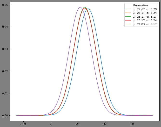
Unusual! Player at index 2 has a greater ordinal even though the player is lower in rank. Okay, maybe the ditribution plots give more explanation?

visualization_data = np.arange(-25, 75, 0.001)
fig = plt.figure(figsize=(10, 8), dpi=80)
fig.patch.set_facecolor("grey")
df.apply(
    lambda row: plt.plot(
        visualization_data,
        norm.pdf(visualization_data, row["mu"], row["sigma"]),
        label=f"μ: {row['mu']: 0.2f}, σ: {row['sigma']: 0.2f}",
    ),
    axis=1,
)
plt.legend(title="Parameters")

<matplotlib.legend.Legend at 0x79208ec85e10>

It looks like players at index 1, 2 and 3, they have almost indentical means. So they overlap each other quite a bit. But if you have a keen eye, you will notice that the green line representing player at index 2 has a higher peak (also known as negative kurtosis in literature). This means the system is overall more confident in player at index 2’s skill.

By default the value of an ordinal is determined by the fomula ‘\(μ - 3σ\)’ which by the empirical rule only allows for the system to be confident upto 99.7%. As such when \(σ\) is still high such as when players have played few games will lead to the overal ordinal fluctuating.

You can curtail this effect for large numbers of matches by using the “Additive Dynamics Factor” \(\tau\) (parameter “tau”) into the models of this library in combination with the limit_sigma parameter.